
Type: Systems Research CS Education Operating Systems
Author: Zirov
Date: 2025-03-30
When multiple processes compete for a single CPU, the scheduler decides who runs, when, and for how long — a deceptively simple problem with profound consequences for performance, fairness, and responsiveness.
Abstract
Modern operating systems routinely manage dozens to thousands of concurrent processes on hardware that may expose only a handful of CPU cores. CPU scheduling is the policy layer that resolves this contention — it decides which ready process gets the processor at any given moment, for how long, and under what conditions it can be preempted. This article covers the foundational scheduling algorithms (FCFS, SJF, SRTF, and Round Robin), derives their performance characteristics analytically using a shared example dataset, and traces how their theoretical models evolved into the schedulers shipping inside Linux and Windows today. It also surfaces the real-world pathologies — starvation, convoy effect, excessive context-switch overhead — that make production scheduling considerably harder than textbook examples suggest. By the end, the reader should be able to reason critically about scheduler trade-offs, implement a simulator in C, and understand why no single algorithm is universally optimal.
Introduction
The Real-World Problem
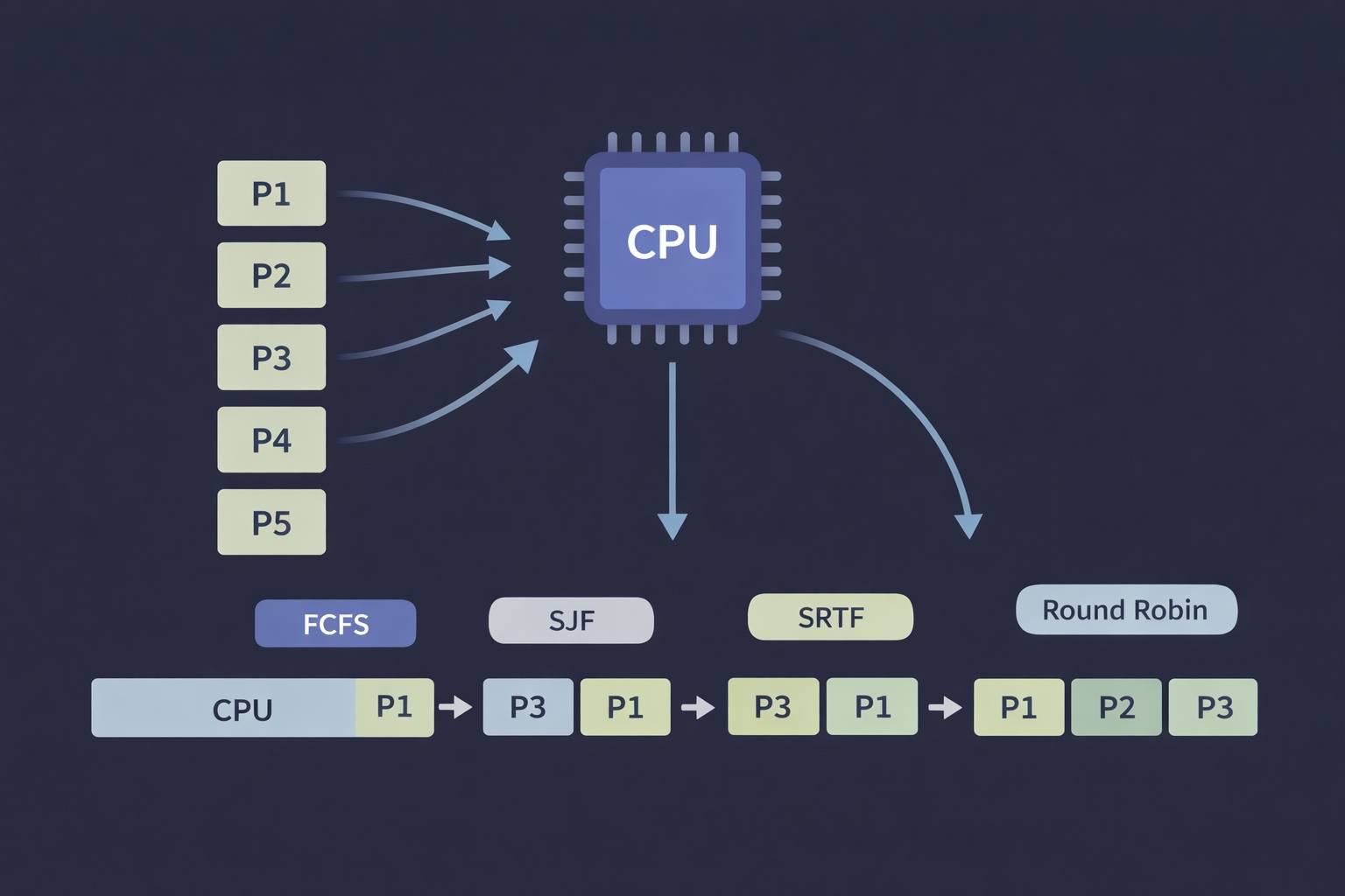
A web server can receive many requests at the same time. Behind the scenes, several processes wait in the ready queue for CPU time to run application logic and generate a response. But since the hardware has a limited number of CPU cores, something has to decide which process runs first.
This is the baseline state of any modern multitasking operating system. Even on a personal laptop, background services, the user interface, browser tabs, antivirus scans, and user applications are all competing for CPU time. The component responsible for managing this competition is the CPU scheduler.
Why It Matters for Performance and Responsiveness
The scheduling policy chosen by an OS has a direct and measurable impact on the user experience. A poorly chosen scheduler can cause an interactive application to freeze for several seconds while a background job monopolizes the CPU. A well-designed one ensures that every process receives timely, fair access to the processor — keeping the system responsive under load. Understanding scheduling is therefore essential not just for OS designers, but for any systems programmer who needs to reason about latency, throughput, and resource contention.
CPU Scheduling
CPU scheduling is the mechanism an operating system uses to determine which process or task gets access to the CPU at a given moment. This is necessary because the CPU can execute only one task at a time, while multiple tasks are usually waiting to run.
Why It Is Necessary
Scheduling is necessary because multiple processes may be ready to run simultaneously while the CPU can execute only one at a time. The operating system must decide which process gets the CPU next, ensuring that the processor does not remain idle and that system resources are used efficiently. Without a scheduling policy, the CPU would either sit idle or execute processes in an arbitrary order, leading to unpredictable and often poor performance.
Goals
As a general rule, the objective of scheduling is to:
- Maximize CPU utilization and processing throughput
- Minimize execution time, waiting time, and response time
- Ensure fairness — no process should be indefinitely denied access to the CPU
- Meet deadlines in real-time systems where timing guarantees are required
Types of Scheduling
Scheduling can be classified into two main types.
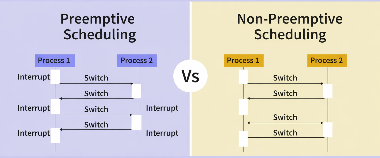
Preemptive
In a preemptive scheduler, the OS can forcibly reclaim the CPU from a running process — typically on a timer interrupt, on the arrival of a higher-priority process, or when a better candidate appears in the ready queue.
If a process with high priority arrives in the ready queue, it does not have to wait for the current process to complete its burst time. Instead, the current process is interrupted in the middle of execution and placed back in the ready queue until the higher-priority process finishes using the CPU. This makes preemptive scheduling flexible, but it increases the overhead associated with switching a process from the running state to the ready state and vice versa.
Algorithms that operate under preemptive scheduling include Round Robin and Shortest Remaining Time First (SRTF). Shortest Job First (SJF) and Priority Scheduling may or may not be preemptive depending on the implementation.
To better understand how preemptive scheduling works, consider the following example with four processes:
| Process | Arrival Time | Burst Time |
|---|---|---|
| P1 | 0 | 7 ms |
| P2 | 2 | 4 ms |
| P3 | 3 | 2 ms |
| P4 | 5 | 3 ms |
At time 0, only P1 has arrived in the ready queue, so the CPU begins executing P1.
At time 2, process P2 arrives. Because the system uses a preemptive scheduling algorithm, the scheduler compares the remaining execution time of P1 with the burst time of P2. Since P2 requires less time, the CPU preempts P1 and starts executing P2.
| Process | Remaining Time |
|---|---|
| P1 | 5 ms |
| P2 | 4 ms |
At time 3, process P3 arrives with an even shorter burst time. The scheduler compares the remaining execution times and selects the shortest one. As a result, P2 is interrupted, and the CPU is assigned to P3.
| Process | Remaining Time |
|---|---|
| P1 | 5 ms |
| P2 | 3 ms |
| P3 | 2 ms |
Process P3 continues executing until it finishes at time 5.
At time 5, P4 arrives. The scheduler now compares the remaining processes:
| Process | Remaining Time |
|---|---|
| P1 | 5 ms |
| P2 | 3 ms |
| P4 | 3 ms |
Since P2 and P4 have the same remaining time, the scheduler selects P2 because it arrived earlier. Therefore, P2 resumes execution and continues until it finishes at time 8.
After P2 completes, the scheduler compares the remaining processes:
| Process | Remaining Time |
|---|---|
| P1 | 5 ms |
| P4 | 3 ms |
The CPU is then allocated to P4, which executes from time 8 to time 11.
Finally, P1 is the only process left in the ready queue, so it resumes execution and finishes at time 16.
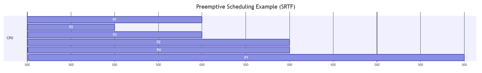
The resulting Gantt Chart is:
Non-Preemptive
In a non-preemptive scheduler, a process runs until it finishes or moves to a waiting state. The OS cannot forcibly take the CPU away from a running process.
Unlike preemptive scheduling, non-preemptive scheduling does not interrupt a process in the middle of execution. Instead, it waits for the process to complete its CPU burst time before allocating the CPU to another process. This eliminates the overhead of context switching mid-burst, but it also means that a high-priority process arriving while a long process is running must wait — making the system less responsive.
To understand how non-preemptive scheduling works, consider the same set of processes used in the previous example:
| Process | Arrival Time | Burst Time |
|---|---|---|
| P1 | 0 | 7 ms |
| P2 | 2 | 4 ms |
| P3 | 3 | 2 ms |
| P4 | 5 | 3 ms |
At time 0, only P1 has arrived in the ready queue, so the CPU starts executing P1.
In non-preemptive scheduling, once a process starts executing, it cannot be interrupted until it finishes its CPU burst. Therefore, even if other processes arrive with shorter burst times, they must wait until the current process completes.
Between time 2 and time 5, processes P2, P3, and P4 arrive in the ready queue. However, P1 continues executing because the scheduler cannot preempt it.
| Process | Arrival Time | Burst Time |
|---|---|---|
| P2 | 2 | 4 ms |
| P3 | 3 | 2 ms |
| P4 | 5 | 3 ms |
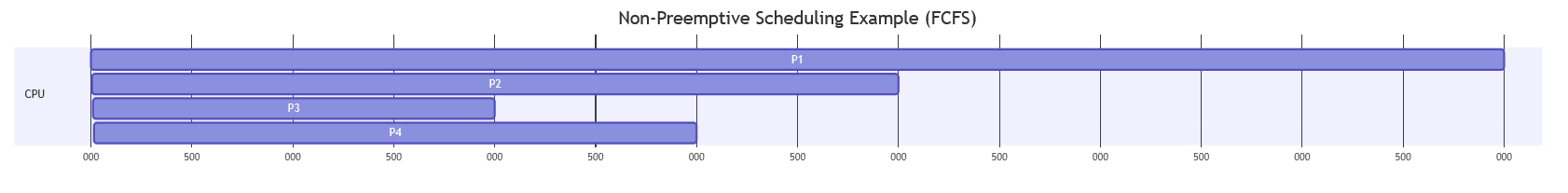
At time 7, P1 finishes execution. The scheduler now selects the next process from the ready queue. Assuming a First Come First Serve (FCFS) order among the waiting processes, P2 is selected because it arrived first.
P2 executes from time 7 to time 11.
After P2 completes, the scheduler selects the next process in the ready queue, which is P3.
P3 executes from time 11 to time 13.
Finally, P4 is the last remaining process in the queue and executes from time 13 to time 16.
The resulting Gantt Chart is:
Scheduling Algorithms
First Come First Served (FCFS)
FCFS is the simplest and most straightforward scheduling algorithm. The principle is exactly as it sounds: processes are executed in the order they arrive, without any prioritization. This method is analogous to standing in a queue at a supermarket checkout — the first person in line is the first to be served.
Advantages
- Trivial to implement (a single FIFO queue)
- No starvation — every process eventually reaches the front
- No parameters to tune
Disadvantages
- Convoy effect: One long CPU-bound process forces all shorter processes behind it to wait, dramatically inflating average waiting time
- Poor average waiting time for mixed workloads
- Zero responsiveness guarantee for interactive processes
Typical Use Cases
- Simple batch processing queues
- Print spoolers
- Foundational building block for more complex schedulers
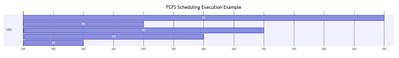
Execution Example
Consider the following set of processes:
| Process | Arrival Time | Burst Time |
|---|---|---|
| P1 | 0 | 6 ms |
| P2 | 1 | 2 ms |
| P3 | 2 | 4 ms |
| P4 | 3 | 3 ms |
| P5 | 4 | 1 ms |
Since FCFS executes processes strictly in the order they arrive, once a process starts executing it runs until completion before the next process begins.
At time 0, only P1 has arrived, so the CPU starts executing P1. Even though P2, P3, P4, and P5 arrive while P1 is running, they must wait in the ready queue.
Execution proceeds as follows:
- P1 executes from 0 → 6
- P2 executes from 6 → 8
- P3 executes from 8 → 12
- P4 executes from 12 → 15
- P5 executes from 15 → 16
The resulting Gantt Chart is:
Implementation in C
#include <stdio.h>

int main() {
    int n, i;
    int at[20], bt[20], wt[20], ct[20], tat[20];
    float wtavg = 0, tatavg = 0;

    printf("Enter the number of processes: ");
    scanf("%d", &n);

    for (i = 0; i < n; i++) {
        printf("Enter arrival time and burst time for process P%d: ", i + 1);
        scanf("%d %d", &at[i], &bt[i]);
    }

    // First process starts immediately at its arrival time
    ct[0]  = at[0] + bt[0];
    tat[0] = ct[0] - at[0];
    wt[0]  = 0;
    tatavg = tat[0];

    for (i = 1; i < n; i++) {
        // If CPU is idle between processes, account for the gap
        ct[i]  = (ct[i - 1] > at[i] ? ct[i - 1] : at[i]) + bt[i];
        wt[i]  = ct[i] - at[i] - bt[i];
        tat[i] = ct[i] - at[i];
        wtavg  += wt[i];
        tatavg += tat[i];
    }

    wtavg  /= n;
    tatavg /= n;

    printf("\n%-10s %-12s %-10s %-14s %-12s %-16s\n",
           "Process", "Arrival_T", "Burst_T", "Complete_T", "Waiting_T", "Turnaround_T");
    for (i = 0; i < n; i++) {
        printf("%-10s %-12d %-10d %-14d %-12d %-16d\n",
               (char[]){'P', '0' + i + 1, '\0'}, at[i], bt[i], ct[i], wt[i], tat[i]);
    }

    printf("\nGantt Chart:\n|");
    for (i = 0; i < n; i++) printf(" P%d |", i + 1);
    printf("\n0");
    for (i = 0; i < n; i++) printf("\t%d", ct[i]);
    printf("\n");

    printf("\nAverage Waiting Time   : %.2f ms\n", wtavg);
    printf("Average Turnaround Time: %.2f ms\n", tatavg);

    return 0;
}
Shortest Job First (SJF)
SJF selects the process in the ready queue with the smallest burst time. It is non-preemptive: once a process starts, it runs to completion. Among processes with equal burst times, FCFS tie-breaking applies.
SJF is provably optimal for minimizing average waiting time among non-preemptive algorithms — but it requires knowing burst times in advance, which is generally impossible in practice. Real systems estimate them from historical CPU usage using exponential averaging.
Advantages
- Minimizes average waiting time among all non-preemptive algorithms
- High throughput for mixed-length workloads
Disadvantages
- Starvation: Long processes may never execute if shorter ones keep arriving
- Requires accurate burst time prediction — estimation error propagates into suboptimal decisions
- Not suitable for interactive workloads in its non-preemptive form
Typical Use Cases
- Batch schedulers where job run-time estimates are available (e.g., HPC clusters with declared job times)
- Database query planners (analogous "shortest query first" heuristics)
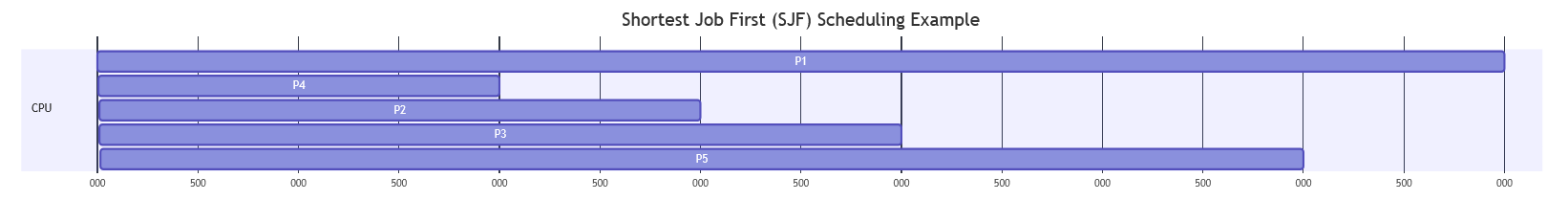
Execution Example
Consider the following set of processes:
| Process | Arrival Time | Burst Time |
|---|---|---|
| P1 | 0 | 7 ms |
| P2 | 1 | 3 ms |
| P3 | 2 | 4 ms |
| P4 | 3 | 2 ms |
| P5 | 4 | 6 ms |
Since SJF always selects the process with the smallest burst time among those currently in the ready queue, scheduling decisions are based on job length rather than arrival order.
At time 0, only P1 has arrived, so the CPU begins executing P1. Because this version of SJF is non-preemptive, P1 continues running until it finishes, even though shorter jobs arrive later.
During the execution of P1, the remaining processes arrive and wait in the ready queue.
At time 7, P1 finishes. The scheduler selects the process with the shortest burst time from the queue:
| Process | Burst Time |
|---|---|
| P2 | 3 ms |
| P3 | 4 ms |
| P4 | 2 ms |
| P5 | 6 ms |
The shortest job is P4, so it executes next. Execution proceeds as follows:
- P1 executes from 0 → 7
- P4 executes from 7 → 9
- P2 executes from 9 → 12
- P3 executes from 12 → 16
- P5 executes from 16 → 22
The resulting Gantt Chart is:
Implementation in C
#include <stdio.h>

int main() {
    int n, i, j, pos;
    int at[20], bt[20], wt[20], ct[20], tat[20], temp_bt[20], temp_at[20], order[20];
    float wtavg = 0, tatavg = 0;
    int current_time = 0, completed = 0;
    int visited[20] = {0};

    printf("Enter the number of processes: ");
    scanf("%d", &n);

    for (i = 0; i < n; i++) {
        printf("Enter arrival time and burst time for process P%d: ", i + 1);
        scanf("%d %d", &at[i], &bt[i]);
        temp_bt[i] = bt[i];
        temp_at[i] = at[i];
    }

    // Non-preemptive SJF: simulate step by step
    int exec_order[20];
    int exec_count = 0;

    while (completed < n) {
        // Find shortest available job at current_time
        int min_bt = 99999, sel = -1;
        for (i = 0; i < n; i++) {
            if (!visited[i] && at[i] <= current_time) {
                if (bt[i] < min_bt) {
                    min_bt = bt[i];
                    sel = i;
                } else if (bt[i] == min_bt && at[i] < at[sel]) {
                    sel = i;
                }
            }
        }

        if (sel == -1) {
            // CPU idle — advance to next arrival
            int next = 99999;
            for (i = 0; i < n; i++)
                if (!visited[i] && at[i] < next) next = at[i];
            current_time = next;
            continue;
        }

        visited[sel]   = 1;
        current_time  += bt[sel];
        ct[sel]        = current_time;
        tat[sel]       = ct[sel] - at[sel];
        wt[sel]        = tat[sel] - bt[sel];
        wtavg         += wt[sel];
        tatavg        += tat[sel];
        exec_order[exec_count++] = sel;
        completed++;
    }

    wtavg  /= n;
    tatavg /= n;

    printf("\n%-10s %-12s %-10s %-14s %-12s %-16s\n",
           "Process", "Arrival_T", "Burst_T", "Complete_T", "Waiting_T", "Turnaround_T");
    for (i = 0; i < n; i++) {
        printf("%-10s %-12d %-10d %-14d %-12d %-16d\n",
               (char[]){'P', '0' + i + 1, '\0'}, at[i], bt[i], ct[i], wt[i], tat[i]);
    }

    printf("\nGantt Chart:\n|");
    for (i = 0; i < exec_count; i++) printf(" P%d |", exec_order[i] + 1);
    printf("\n");

    printf("\nAverage Waiting Time   : %.2f ms\n", wtavg);
    printf("Average Turnaround Time: %.2f ms\n", tatavg);

    return 0;
}
Shortest Remaining Time First (SRTF)
SRTF is the preemptive version of SJF. Whenever a new process arrives, the scheduler compares its burst time against the remaining burst time of the currently running process. If the newcomer is shorter, it immediately preempts the current process.
SRTF is theoretically optimal for minimizing average waiting time among all scheduling algorithms — preemptive or otherwise — for the same reasons SJF is optimal in the non-preemptive case.
Advantages
- Theoretically optimal average waiting time
- Short jobs get immediate service regardless of when they arrive
Disadvantages
- Starvation of long processes can be severe
- Requires continuous tracking of remaining burst time
- High context-switch frequency increases overhead
- Burst time prediction error is more damaging than in SJF
Typical Use Cases
- Theoretical baseline for evaluating other algorithms
- Approximated in systems with accurate CPU profiling (some batch schedulers)
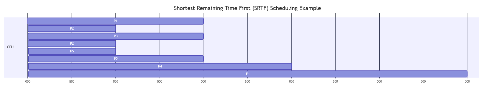
Execution Example
Consider the following set of processes:
| Process | Arrival Time | Burst Time |
|---|---|---|
| P1 | 0 | 7 ms |
| P2 | 2 | 4 ms |
| P3 | 3 | 2 ms |
| P4 | 5 | 3 ms |
| P5 | 6 | 1 ms |
At time 0, only P1 has arrived in the ready queue, so the CPU starts executing P1.
At time 2, P2 arrives. The scheduler compares the remaining time of P1 (5 ms) with the burst time of P2 (4 ms). Since P2 is shorter, it preempts P1 and begins execution.
At time 3, P3 arrives with a burst time of 2 ms. The scheduler compares all remaining processes:
| Process | Remaining Time |
|---|---|
| P1 | 5 ms |
| P2 | 3 ms |
| P3 | 2 ms |
Since P3 has the shortest remaining time, P2 is preempted and the CPU is assigned to P3.
P3 executes until time 5, when it finishes. At this moment P4 arrives.
Remaining processes:
| Process | Remaining Time |
|---|---|
| P1 | 5 ms |
| P2 | 3 ms |
| P4 | 3 ms |
The scheduler selects P2 (tie broken by earlier arrival), which executes from time 5 to time 6.
At time 6, P5 arrives with a burst time of 1 ms, which is shorter than the remaining time of P2 (2 ms). Therefore, P2 is preempted again, and the CPU is allocated to P5.
Execution continues as follows:
- P1 executes from 0 → 2
- P2 executes from 2 → 3
- P3 executes from 3 → 5
- P2 executes from 5 → 6
- P5 executes from 6 → 7
- P2 executes from 7 → 9
- P4 executes from 9 → 12
- P1 executes from 12 → 17
The resulting Gantt Chart is:
Implementation in C
#include <stdio.h>

int main() {
    int n, i;
    int at[20], bt[20], remaining[20], wt[20], ct[20], tat[20];
    float wtavg = 0, tatavg = 0;
    int completed = 0, current_time = 0, min_rem, sel;
    int done[20] = {0};

    printf("Enter the number of processes: ");
    scanf("%d", &n);

    for (i = 0; i < n; i++) {
        printf("Enter arrival time and burst time for process P%d: ", i + 1);
        scanf("%d %d", &at[i], &bt[i]);
        remaining[i] = bt[i];
    }

    while (completed < n) {
        min_rem = 99999;
        sel     = -1;

        for (i = 0; i < n; i++) {
            if (!done[i] && at[i] <= current_time && remaining[i] < min_rem) {
                min_rem = remaining[i];
                sel     = i;
            }
        }

        if (sel == -1) {
            current_time++;
            continue;
        }

        remaining[sel]--;
        current_time++;

        if (remaining[sel] == 0) {
            done[sel]  = 1;
            ct[sel]    = current_time;
            tat[sel]   = ct[sel] - at[sel];
            wt[sel]    = tat[sel] - bt[sel];
            wtavg     += wt[sel];
            tatavg    += tat[sel];
            completed++;
        }
    }

    wtavg  /= n;
    tatavg /= n;

    printf("\n%-10s %-12s %-10s %-14s %-12s %-16s\n",
           "Process", "Arrival_T", "Burst_T", "Complete_T", "Waiting_T", "Turnaround_T");
    for (i = 0; i < n; i++) {
        printf("%-10s %-12d %-10d %-14d %-12d %-16d\n",
               (char[]){'P', '0' + i + 1, '\0'}, at[i], bt[i], ct[i], wt[i], tat[i]);
    }

    printf("\nAverage Waiting Time   : %.2f ms\n", wtavg);
    printf("Average Turnaround Time: %.2f ms\n", tatavg);

    return 0;
}
Round Robin (RR)
Round Robin assigns each process a fixed time quantum (also called a time slice). Processes execute in FIFO order, but no process runs for more than one quantum before being preempted and moved to the back of the ready queue. If a process completes before its quantum expires, the CPU is immediately given to the next process.
Round Robin is the backbone of modern interactive schedulers. Its fairness is structural — every process gets CPU time within at most (n − 1) × quantum time units.
Advantages
- Strong fairness guarantee — no process waits more than
(n-1) × Qtime units - Good response time for interactive workloads
- No starvation possible
Disadvantages
- Average waiting time is often higher than SJF for identical workloads
- Performance is sensitive to quantum size:
- Too small: Context-switch overhead dominates useful work
- Too large: Degenerates toward FCFS behavior
- Higher context-switch cost than non-preemptive algorithms
Typical Use Cases
- General-purpose desktop and server operating systems (as a component of more complex schedulers)
- Time-sharing systems where equal treatment of interactive users is the primary goal
- Virtual machine CPU time-sharing between guests
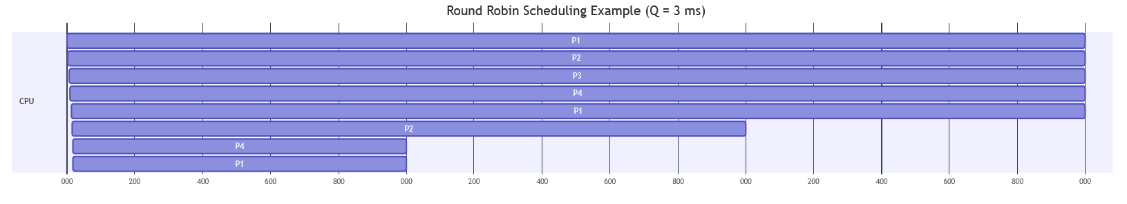
Execution Example
Consider the following processes and a time quantum (Q) = 3 ms:
| Process | Arrival Time | Burst Time |
|---|---|---|
| P1 | 0 | 7 ms |
| P2 | 1 | 5 ms |
| P3 | 2 | 3 ms |
| P4 | 3 | 4 ms |
At time 0, only P1 is in the ready queue, so it begins execution. Since the quantum is 3 ms, P1 executes for 3 ms and is then preempted because it still has remaining burst time.
Remaining processes after the first quantum:
| Process | Remaining Time |
|---|---|
| P1 | 4 ms |
| P2 | 5 ms |
| P3 | 3 ms |
| P4 | 4 ms |
Execution proceeds in FIFO order, with each process receiving at most one quantum per turn:
- P1 executes from 0 → 3 (remaining: 4)
- P2 executes from 3 → 6 (remaining: 2)
- P3 executes from 6 → 9 (finishes)
- P4 executes from 9 → 12 (remaining: 1)
- P1 executes from 12 → 15 (remaining: 1)
- P2 executes from 15 → 17 (finishes)
- P4 executes from 17 → 18 (finishes)
- P1 executes from 18 → 19 (finishes)
The resulting Gantt Chart is:
Implementation in C
#include <stdio.h>

int main() {
    int n, i, quantum;
    int at[20], bt[20], remaining[20], wt[20], ct[20], tat[20];
    float wtavg = 0, tatavg = 0;
    int current_time = 0, completed = 0;
    int queue[200], front = 0, rear = 0;
    int in_queue[20] = {0};

    printf("Enter the number of processes: ");
    scanf("%d", &n);

    for (i = 0; i < n; i++) {
        printf("Enter arrival time and burst time for process P%d: ", i + 1);
        scanf("%d %d", &at[i], &bt[i]);
        remaining[i] = bt[i];
    }

    printf("Enter the time quantum: ");
    scanf("%d", &quantum);

    // Enqueue process 0 if it arrives at time 0
    for (i = 0; i < n; i++) {
        if (at[i] == 0) {
            queue[rear++] = i;
            in_queue[i]   = 1;
        }
    }

    while (completed < n) {
        if (front == rear) {
            // Queue empty — advance time to next arrival
            current_time++;
            for (i = 0; i < n; i++) {
                if (!in_queue[i] && remaining[i] > 0 && at[i] <= current_time) {
                    queue[rear++] = i;
                    in_queue[i]   = 1;
                }
            }
            continue;
        }

        int p = queue[front++];

        int run_time = (remaining[p] < quantum) ? remaining[p] : quantum;
        current_time   += run_time;
        remaining[p]   -= run_time;

        // Enqueue newly arrived processes during this slice
        for (i = 0; i < n; i++) {
            if (!in_queue[i] && remaining[i] > 0 && at[i] <= current_time) {
                queue[rear++] = i;
                in_queue[i]   = 1;
            }
        }

        if (remaining[p] == 0) {
            ct[p]    = current_time;
            tat[p]   = ct[p] - at[p];
            wt[p]    = tat[p] - bt[p];
            wtavg   += wt[p];
            tatavg  += tat[p];
            completed++;
        } else {
            // Re-enqueue for the next round
            queue[rear++] = p;
        }
    }

    wtavg  /= n;
    tatavg /= n;

    printf("\n%-10s %-12s %-10s %-14s %-12s %-16s\n",
           "Process", "Arrival_T", "Burst_T", "Complete_T", "Waiting_T", "Turnaround_T");
    for (i = 0; i < n; i++) {
        printf("%-10s %-12d %-10d %-14d %-12d %-16d\n",
               (char[]){'P', '0' + i + 1, '\0'}, at[i], bt[i], ct[i], wt[i], tat[i]);
    }

    printf("\nAverage Waiting Time   : %.2f ms\n", wtavg);
    printf("Average Turnaround Time: %.2f ms\n", tatavg);

    return 0;
}
Algorithm Comparison
| Algorithm | Type | Fairness | Complexity | Starvation Risk | Optimal For |
|---|---|---|---|---|---|
| FCFS | Non-preemptive | Arrival-order fair | O(1) enqueue | None | Simple batch workloads |
| SJF | Non-preemptive | Biased toward short jobs | O(n) selection | Long processes | Batch with known burst times |
| SRTF | Preemptive | Biased toward short jobs | O(n) on arrival | Long processes | Minimizing avg WT (theoretical) |
| Round Robin | Preemptive | Time-equal | O(1) | None | Interactive, time-sharing |
Comparative Example
To better understand the behavior of each scheduling algorithm, consider the same set of processes executed under different schedulers.
| Process | Arrival Time | Burst Time |
|---|---|---|
| P1 | 0 | 7 ms |
| P2 | 1 | 4 ms |
| P3 | 2 | 2 ms |
| P4 | 3 | 3 ms |
| P5 | 4 | 1 ms |
FCFS
Processes execute strictly in arrival order.
Execution order:
P1 → P2 → P3 → P4 → P5
- Avg Waiting Time: 9.2 ms
- Avg Turnaround Time: 12.6 ms
SJF (Non-Preemptive)
After the first process finishes, the scheduler selects the shortest job in the ready queue.
Execution order:
P1 → P5 → P3 → P4 → P2
- Avg Waiting Time: 7.0 ms
- Avg Turnaround Time: 10.4 ms
SRTF (Preemptive SJF)
Processes can interrupt the currently running job if they have a shorter remaining time.
Execution order (timeline):
P1 → P3 → P5 → P3 → P4 → P2 → P1
- Avg Waiting Time: 3.6 ms
- Avg Turnaround Time: 7.0 ms
Round Robin (Q = 3)
Each process runs for at most 3 ms before being preempted and moved to the back of the queue.
Execution order:
P1 → P2 → P3 → P4 → P5 → P1 → P2 → P4 → P1
- Avg Waiting Time: 9.0 ms
- Avg Turnaround Time: 12.4 ms
Summary
| Algorithm | Avg WT | Avg TAT | Characteristic |
|---|---|---|---|
| FCFS | 9.2 | 12.6 | Simple but prone to convoy effect |
| SJF | 7.0 | 10.4 | Better for short jobs |
| SRTF | 3.6 | 7.0 | Best average waiting time |
| RR (Q=3) | 9.0 | 12.4 | Fair and responsive |
The results confirm the theoretical expectations: SRTF delivers the lowest average waiting time, but at the cost of frequent preemptions and potential starvation of long jobs. Round Robin provides strong fairness with no starvation risk, though its average waiting time is comparable to FCFS for this workload. SJF sits in the middle — better than FCFS without the overhead of continuous preemption.
Real OS Scheduling
The algorithms covered so far are clean abstractions. Real OS schedulers are more complex — they must handle hundreds of concurrent processes, NUMA topologies, heterogeneous core types, energy management, and security isolation. Here is how the two dominant platforms approach the problem.
Linux: Completely Fair Scheduler (CFS)
Introduced: Linux 2.6.23 (2007), replacing the O(1) scheduler.
Fairness Model
CFS does not use time slices in the traditional sense. Instead, it tracks each process's virtual runtime (vruntime) — the amount of CPU time it has consumed, normalized by its priority weight. The scheduler always picks the process with the lowest vruntime — the one that has received the least CPU time relative to its entitlement.
This creates a fair allocation without requiring explicit time quantum bookkeeping: a process that has been waiting automatically accumulates a lower vruntime, making it the preferred candidate.
Red-Black Tree Structure
Ready processes are stored in a self-balancing red-black tree, indexed by vruntime. The leftmost node (minimum vruntime) is cached for O(1) access. When a process is selected to run, it is removed from the tree; when it is preempted, its updated vruntime is inserted back in the correct position in O(log n).
This gives CFS O(log n) scheduling decisions and O(1) best-candidate lookup — efficient even with thousands of runnable tasks.
Priority Integration
Linux nice values (−20 to +19) are translated into load weight multipliers. A process with nice=-20 has approximately 10× the weight of a nice=0 process. CFS advances vruntime more slowly for high-weight processes, giving them more real CPU time per unit of virtual time.
Key Characteristics
| Property | CFS Value |
|---|---|
| Algorithm base | Weighted fair queuing |
| Data structure | Red-black tree (per run queue, per NUMA node) |
| Preemption | Yes, on tick and on wakeup |
| Default time slice | Dynamic (scales with number of runnable tasks) |
| Starvation | Prevented by design (vruntime normalization) |
Windows: Priority-Based Scheduler with Dynamic Feedback
Priority Model
Windows uses a 32-level priority scheme (0–31). Real-time processes occupy levels 16–31; normal user processes occupy levels 1–15; the idle thread sits at level 0. The kernel always runs the highest-priority ready thread. Among equal priorities, Round Robin with a time quantum applies.
Multi-Level Feedback Queues
Windows maintains a separate ready queue for each of the 32 priority levels. The scheduler scans from level 31 downward to find the highest non-empty queue. This gives O(1) scheduling decisions for the common case.
Dynamic Priorities
To prevent starvation of lower-priority threads and to reward I/O-bound behavior, Windows applies temporary priority boosts:
- A thread woken from I/O wait receives a boost proportional to the I/O type (disk: +1, keyboard: +6, etc.)
- A thread that has not run for a long time (starvation detection) receives a temporary boost to level 15 for two quanta
- Foreground application threads receive a larger quantum multiplier (configurable, typically 3×)
Key Characteristics
| Property | Windows Value |
|---|---|
| Algorithm base | Preemptive multi-level priority + RR within level |
| Priority levels | 32 (0=idle, 1–15=normal, 16–31=real-time) |
| Quantum | Variable (foreground: ~60–120ms, background: ~20–40ms) |
| Starvation mitigation | Aging-based priority boost |
| API | SetThreadPriority(), SetPriorityClass() |
Conclusion
CPU scheduling sits at the intersection of theory and engineering pragmatism. The classical algorithms — FCFS, SJF, SRTF, and Round Robin — define a clean design space with well-understood trade-offs: you can optimize for minimum average waiting time (SRTF), for fairness (RR), or for simplicity (FCFS), but not all three simultaneously.
Real schedulers are composites. Linux CFS applies weighted fair queuing with an elegant vruntime abstraction that eliminates starvation while accommodating priorities. Windows combines strict priority preemption with dynamic feedback to balance responsiveness for interactive threads against throughput for background work. Both systems have evolved significantly over decades precisely because the problem is genuinely hard — workloads are diverse, hardware is heterogeneous, and the cost of a wrong decision scales with the number of users sharing the machine.
For the systems programmer, the practical takeaways are:
- Profile before assuming. The scheduler that looks optimal on paper may behave differently under your specific workload's arrival and burst distributions.
- Match the scheduler to the workload class. Batch jobs, interactive processes, and real-time tasks have fundamentally different requirements and belong in different scheduling classes.
- Respect the overhead model. Context switches are not free. Spinning up thousands of threads to "maximize parallelism" on a 4-core machine will often be slower than a smaller, carefully scheduled pool.
- Understand the tools your OS gives you.
nice,taskset,cgroups,SCHED_FIFO,SCHED_RR,SCHED_DEADLINE— these are production handles on the scheduler that every senior engineer should be comfortable reaching for.
Scheduling is not a solved problem. Multi-core NUMA machines, heterogeneous CPU architectures, and the pressure to reduce energy consumption continue to push the state of the art. The foundational algorithms in this article are the vocabulary — the real sentences are still being written.
References
- Silberschatz, A., Galvin, P. B., & Gagne, G. — Operating System Concepts, 10th ed. (Wiley, 2018)
- Tanenbaum, A. S. — Modern Operating Systems, 4th ed. (Pearson, 2014)
- Linux CFS Scheduler Documentation
- Linux
sched(7)man page - Jones, M. T. — Inside the Linux Scheduler (IBM Developer, 2009)
- Windows Scheduling — Microsoft Docs
- Molnar, I. — CFS Scheduler Design (kernel.org, 2007)